Periodic analyses of weather and climate will be posted here, with links to previous editions at the bottom. Remember to click on the image if you need to zoom in (especially important in this blog entry!).
There is a lot of weather data available online for free to the general public (I won't get into the sites where one must pay for data). There are a few websites that are particularly outstanding, but they require various degrees of skill and knowledge with accessing the data.
1. National Weather Service (NWS):
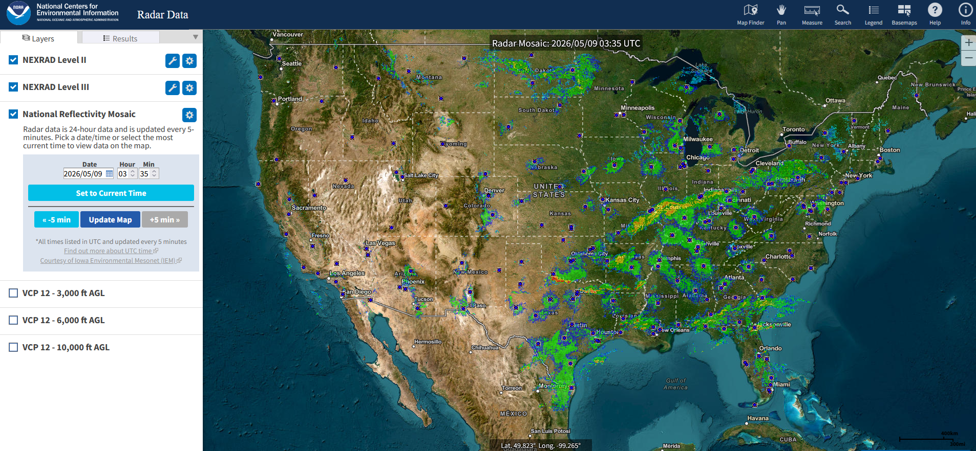
Of course, the National Weather Service (https://www.weather.gov/) has a lot of data available, though the focus is on recent data, such as satellite, radar, and surface observations. A first time user of the site will find the data to be a bit cumbersome, but once you know where to find the data (both in the near-present and past), you will be able to get a wealth of information. The National Weather Service has 122 Weather Forecast Offices (WFOs), and most of them have similar websites (though not entirely so; the "Climate and Past Weather" menu pulldowns vary considerably between offices). Note that this is all separate from the National Centers for Environmental Information (NCEI, https://www.ncei.noaa.gov/), also a part of the National Oceanic and Atmospheric Administration (NOAA), which has advertises storing 229 terabytes of data every month (as of May 2026), but has a steep learning curve for beginners. I will mostly bypass the NCEI website here, though radar reflectivity data (https://www.ncei.noaa.gov/maps/radar/) that they have for the United States is really quite handy and easy to use, and you can zoom in easily. The link goes to a real-time image, but if you type in the year (instead of using the selection tool pulldown), you can get radar data back to 1995. If you wish to dive deeper, go click on the spoke wheels for the "Level 2" and "Level 3" products, though that menu is not as easy to use as the national reflectivity images. Here's a sample image of the live reflectivity data:
A few of my favorite ways to get data from an NWS site include the daily and monthly climate data and recent observations:
If you wish to view a whole month's worth of data at a time for a weather station of your choice, you can go to the xmACIS2 website, which has a moderate learning curve. Or, for more intuitive reference, you can go to any of the NWS individual office pages (the example I show is from NWS San Diego, but each office has a link like this in a similar location on the screen.
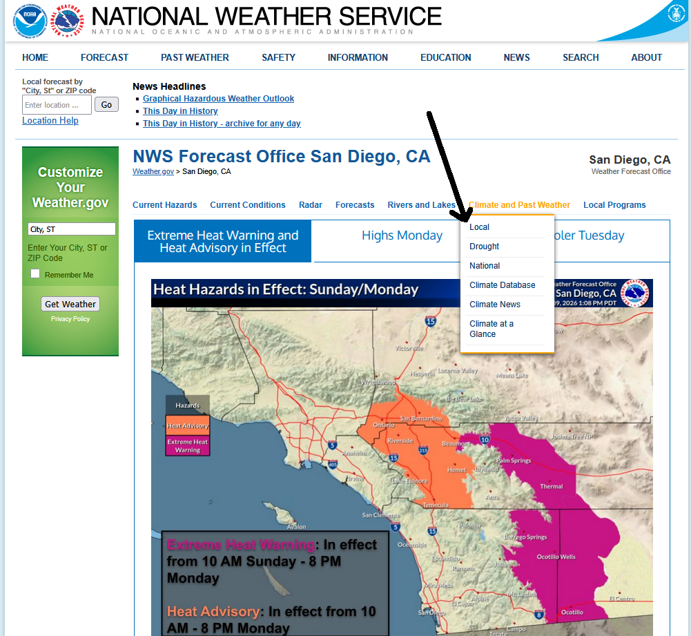
After you click "Climate and Past Weather", you will get a pulldown, with one of them being "Local" (though sometimes just clicking "Climate and Past Weather" will work). You then get something like this:
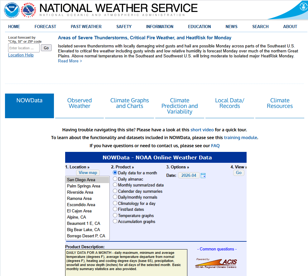
There are numerous tabs here, but I will focus on the first one, "NOWData". This is where you can find the daily data for a month. For locations, if you see something like "San Diego Area" without a specific station selected, then that could cover multiple locations within the city or area, but it will always be whatever was the official record for its time (which, for "San Diego Area", has been San Diego International Airport (formerly known as "Lindbergh Field") since 1 Jul 1939; before then the data were taken downtown.
So is this not strange enough yet (despite the title)? Well, yes, so I will pick a very "strange" month--the month where San Diego had its all-time record high (September 1963).
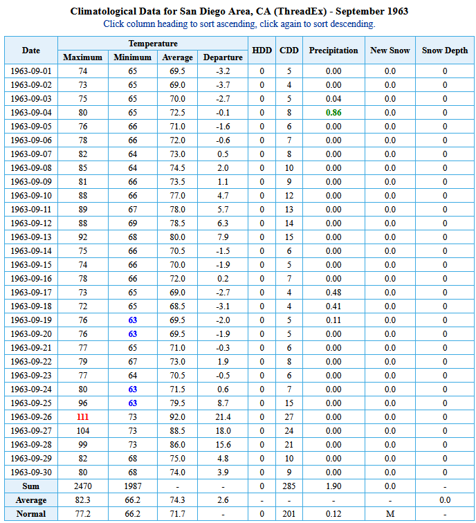
Small detail: I clicked "Enlarge Data" to see the entire month all as once. But otherwise, one can see the high temperature of 111 F (44 C) on 26 Sep 1963 (the red color indicates the warmest for that month), which makes San Diego one of the few locations in the 48 contiguous US states ("CONUS") which has had its all-time high temperature in (calendar) autumn versus summer (all the other sites with this distinction are in coastal California, coastal Oregon, Texas, or Florida). California cities included Los Angeles (both LAX and downtown), Long Beach, Oxnard, Eureka, Oceanside, and perhaps most notably, Imperial Beach, which reached its highest temperature ever of 99 F (37 C) on 4 Nov 1976, the latest date of the year in the CONUS for its all-time highest temperature (I will show how I retrieved that a little later). Outside of the CONUS, Hawaii actually had a station with its highest temperature ever in December, with several other stations with occurrences in November.
There were some other unusual events in September 1963. 1.90" (48 mm) of monthly rainfall is not something normally encountered in San Diego (this was the second wettest September in San Diego, after 1939, which had multiple tropical storms in or close to southern California, including a famous (unnamed) one making landfall near Long Beach). There was measurable rainfall on five days in September 1963, including three days in a row from 17-19 Sep 1963, due to the remnants of Tropical Storm Kathleen. Now let's look at monthly summarized data (which answered a lot of questions that the media and others had for the National Weather Service which I worked there):
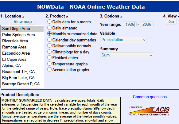
Suppose we wanted to see the precipitation for each month for the past 100 years at San Diego. We would select "Monthly Summarized Data" for the product and "Precipitation" for the variable, while making sure we have 100 years (1926-2026) selected. We would get a lot of data (just showing the top bit here):
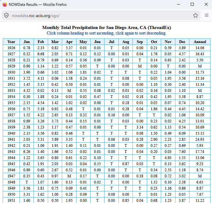
First, note that "M" stands for "Missing" (with xmACIS2, you can actually control what constitutes as "Missing" based on how many daily observations can be missing before the monthly total is missing, but not here), and "T" stands for "Trace" or less than 0.01" of precipitation. But what if you wish to see (using the above example) the wettest Septembers in the past 100 years in San Diego? That's actually easy--just click on the month ("Sep") twice to see the greatest values at the top as it will be ordered far highest to lowest (clicking it once will give you the ordering from lowest to highest).
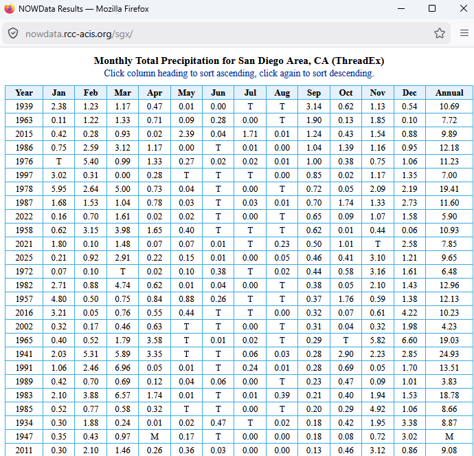
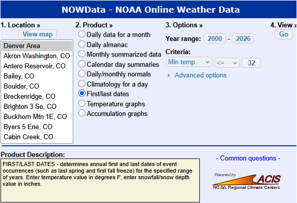
And like mentioned above, 1939 was the wettest September, and 1963 was #2. If you play around with this more, you'll be able to find highest and lowest average temperatures for months, heating degree days (HDDs), etc.--that's your "homework assignment!" Before we jump to other data sources, you can also find the first and last dates of a particular event, either high temperature, low temperature or even snowfall (for some sites). The example below is for Denver's first and last day of the year with a minimum temperature at or below freezing:
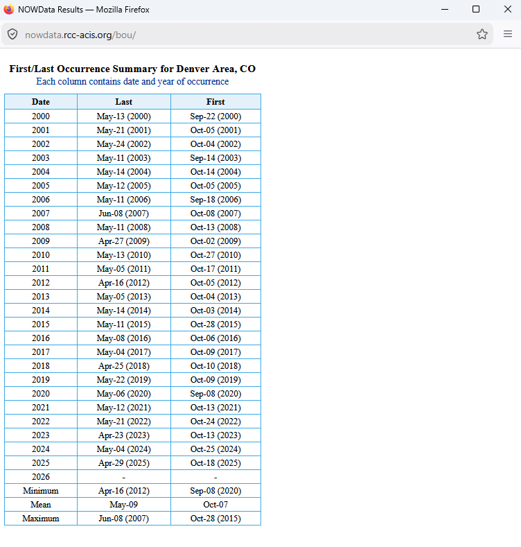
And now the data for this rather unusual climate, including a very late freeze (at least at Denver International Airport) on 8 Jun 2007 and a very early freeze on 8 Sep 2020, literally one day after a high temperature of 93 F (34 C) and three days after a high temperature of 101 F (38 C):
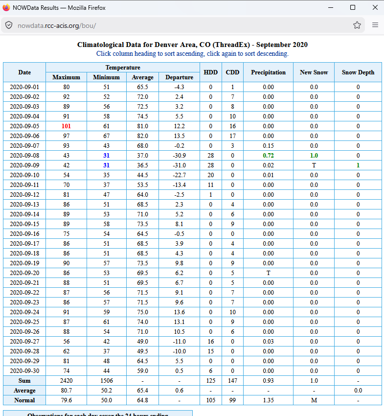
OK, September 2020 was such a crazy month in Denver, that it's worth looking at the monthly chart (including numerous occurrences of high temperatures in the upper 80s to lower 90s after the freeze, and the freeze was even accompanied by snow):
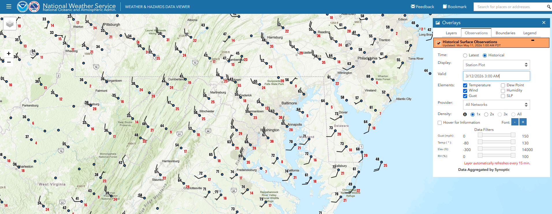
We will have one last look at data on an NWS page before looking elsewhere. You can get a map of surface observations, both in realtime and using historical data (mostly going back to the late 1990s, though with considerably fewer data points when viewing maps of older data). This map is called the Weather and Hazards Data Viewer and contains more than just the surface observations (watches and warnings can be shown as well), but we will focus on the observations here. From most NWS office websites, you can get there by one of the selections (usually "observations") under the "Current Conditions" pulldown (the raw page for the national Weather and Hazards Data Viewer doesn't automatically post the observations, like for temperatures or clouds).
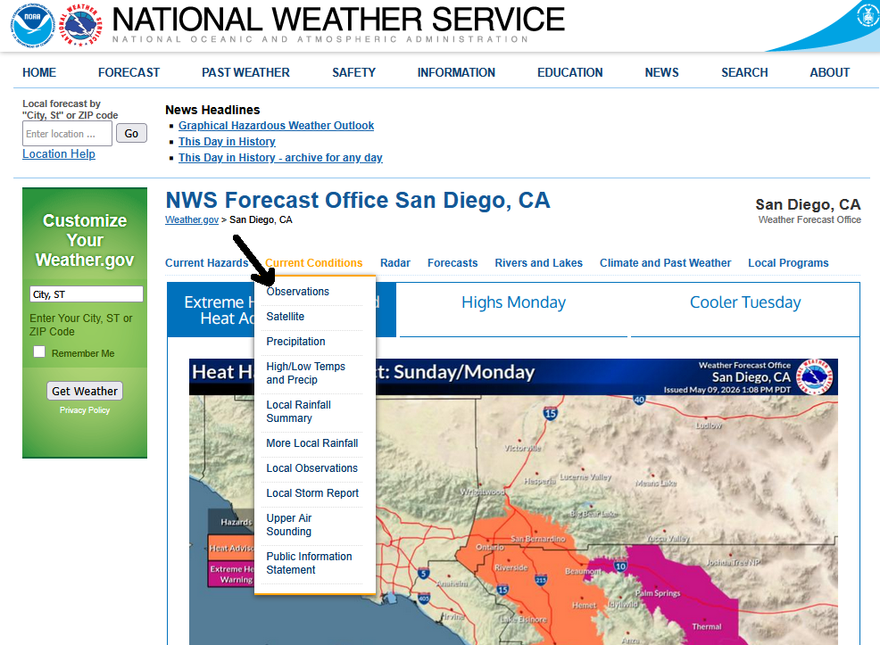
You will initally get something like this (remember to click on the image if it's not big enough on your screen):
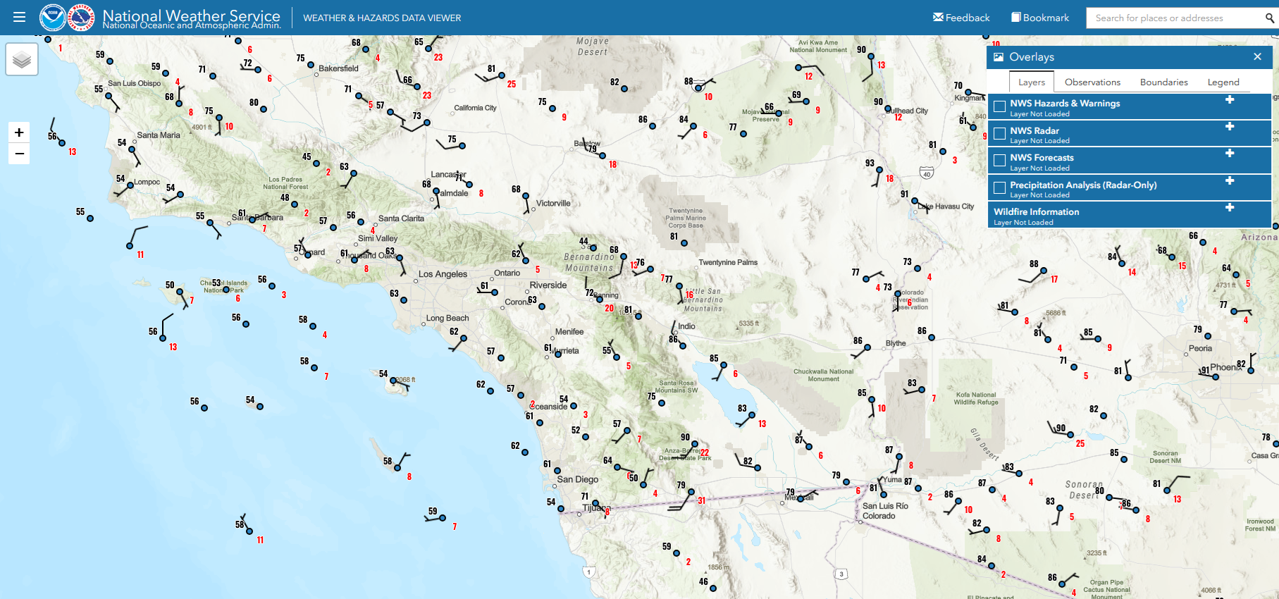
You can look far beyond your local area (actually the entire globe if you zoom out), and there is excellent zooming capability, great for locations with a high density of observations, such as southern Califonria or Switzerland.
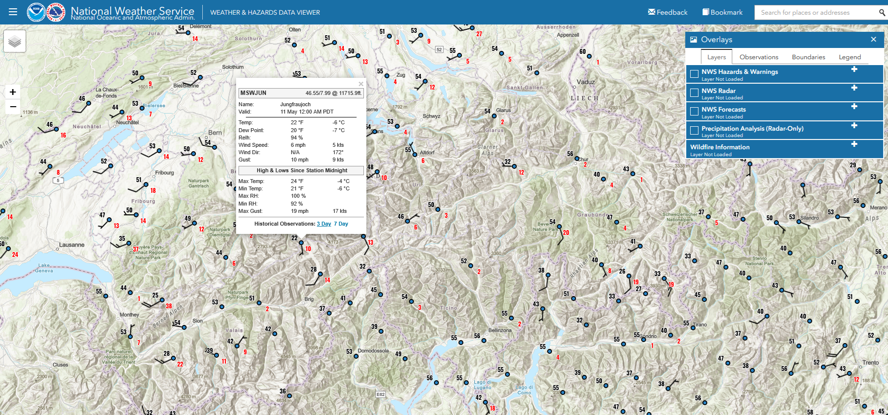
You can then click on a spot to see a table of observations for recent days (up to a month if you know how to rig this). I'll left-click on that 22 F/-6 C reading in Jungfraujoch, Switzerland, considerably colder than surrounding locations due to its high elevation location (around 3600 meters/11700 feet above sea level) for some basic information, then click on "3 Day" for the observations of the past three days.
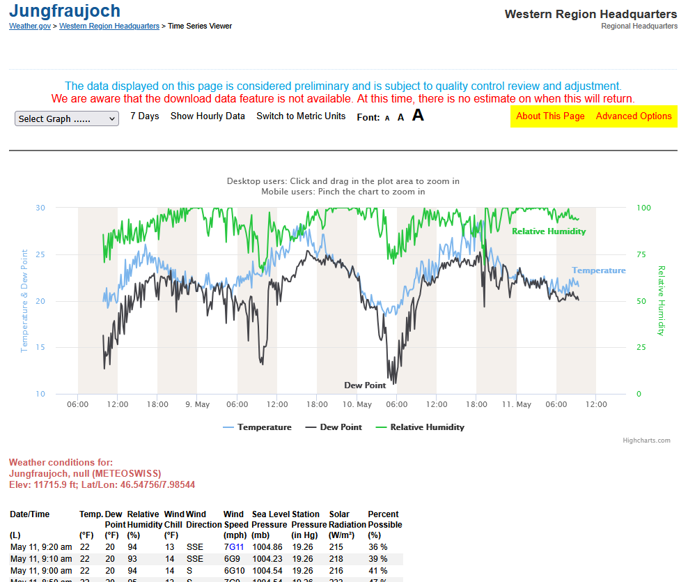
You can view a nice graph (with customizations) of recent weather elements, like temperature, and then see the tabular format below (with a lot of data if you scroll down). While the "published" options are viewing the data for the past 3 or 7 days, you can jimmy this to give you up to 30 days worth of data by taking the URL, in this case https://www.weather.gov/wrh/timeseries?site=MSWJUN&hours=72, and substituting the 72 with 720 (720 hours = 30 days, the limit).
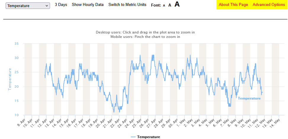
Too much stuff on the graph? You can simply it by selecting just "Temperature" or whatever variable you wish to view (in this case, back 720 hours):
Back to the maps and viewing historical (versus current) data, you will want to select "Observations", then "Historical" in the pulldown to see old data. In this case, we will look at the Mid-Atlantic when a strong cold front moved through the area very early in the morning on 12 Mar 2026. Temperatures ranged from 30 to the mid 70s in the region, and Washington, DC ended up with snow later that day (despite being in the 70s shortly after midnight).
And one last thing, the NWS has a Daily Weather Maps page which has a few basic maps for a quick overview each day: https://www.wpc.ncep.noaa.gov/dailywxmap/.
2. xmACIS2:
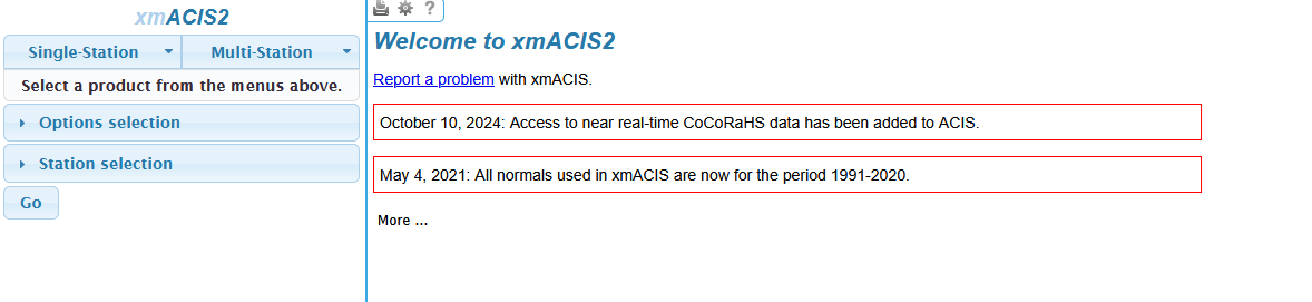
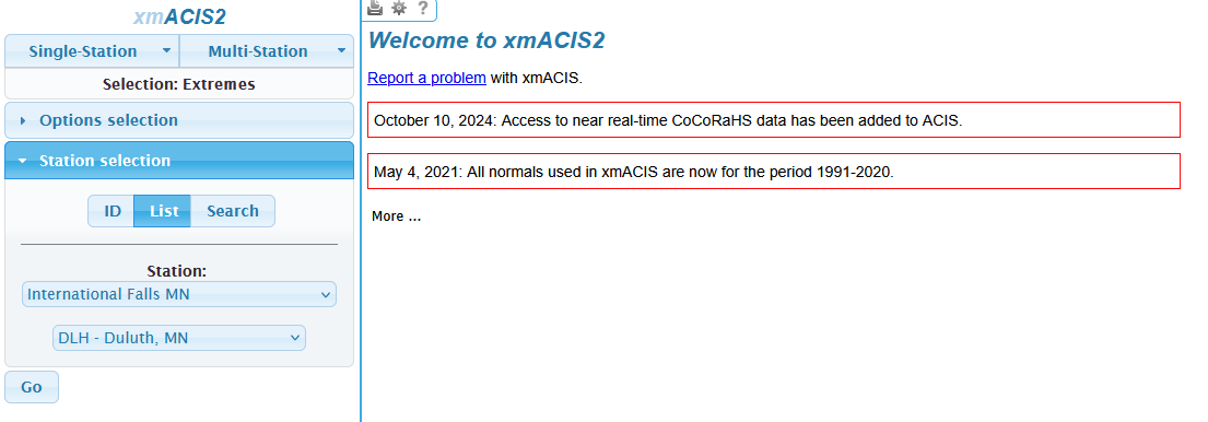
"XMACIS" is a website (https://xmacis.rcc-acis.org/) geared towards meteorologists who are already familiar with the structure of the National Weather Service. Some of the products found in XMACIS appear in the above climate pages of the National Weather Service, but XMACIS has more capabilities for data retrieval. There is kind of a clue that this is for more technical users by the minimalist main page:
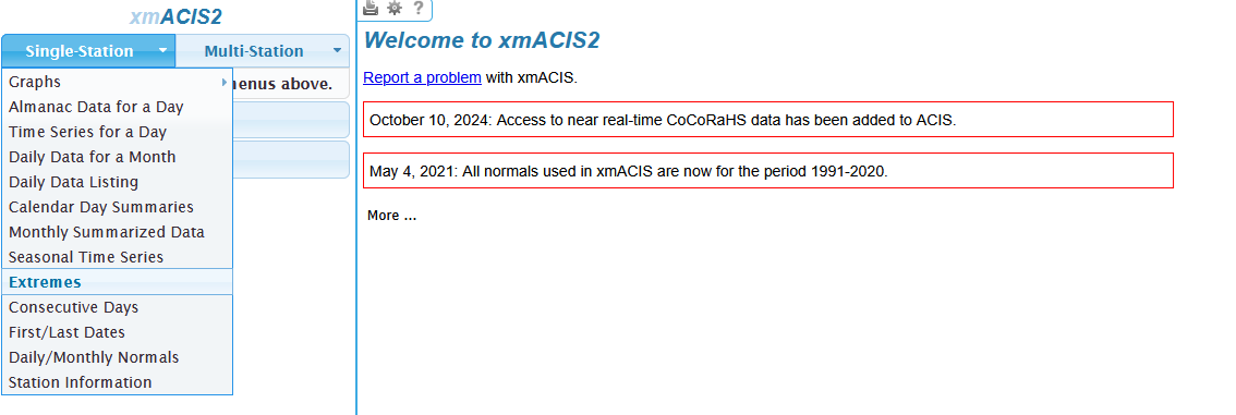
Let's start out with what I consider the most exciting part--the extremes:
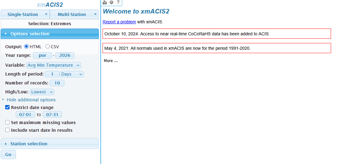
Let's suppose we want to find the lowest overnight low temperatures ever in International Falls, Minnesota. We would select "Avg Min Temperature" for the variable, but making sure the length of period is one day; otherwise, we will be averaging multiple consecutive days together. See? This is aimed at technical users. Side note: "por" stands for "period of record" meaning "por" will go back to the earliest data available. There are some additional options too, such as restricting the date range (so you could have the coldest nights but only in July by setting the date range from 07-01 to 07-31; example for this is below).
The hard part is selecting the location, unless you're familiar with the NWS office structure and office code name. When you click on "Station Selection", you probably won't find the location you're looking for in the station pulldown. Thus, you will either have to search for the station (clicking on "Search" versus the default "List") which will give you a variety of stations nearby, not just the station you're looking for. Or, you must select the office (first) in the second selection before selecting the station in the first selection. For example, one must know to look for DLH - Duluth, MN (the NWS office that covers International Falls) before selecting International Falls:
But once you get through all of that, the fun begins! Here are the results of the ten coldest nights ever in July at International Falls (listed in degrees Fahrenheit):
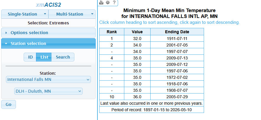
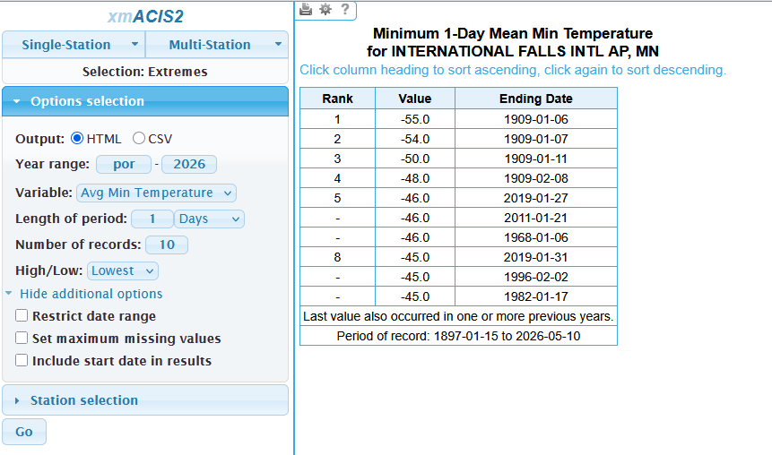
It can get quite chilly there even in July. But here are the brutal results for any time of year (definitely not my kind of weather, either for comfort or gardening!):
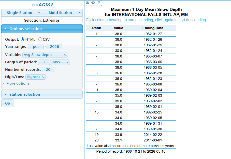
Using the same technique, you can also get the days with the greatest reported snow depth (note it can sometimes be difficult to get an accurate snow depth--or snowfall for that matter--especially with a lot of wind). There were several days in January 1982 in International Falls with 38 inches (97 cm), and a lot of consecutive days overall, so we will look at the top 20 instead of the top 10:
Once you're used to XMACIS, then it gets more intuitive. The key is to practice, if getting this sort of meteorological data is what you wish to do. And, yes, it can get more complicated, as we will see when we select "Multi Station" and can view very specific data covering a large area. Our example will be for the highest temperatures ever reported in the southwestern US (plus a few stations in northwestern Mexico as XMACIS covers some other parts of North America, though it's nowhere close to being global). Just select the "Multi Station" pulldown, then select "Multi-Station Extremes". For a change, we will do a map, but otherwise the selections will be similar to what we've chosen before.
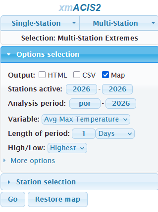
And the final product (kind of a mess, so one must zoom in):
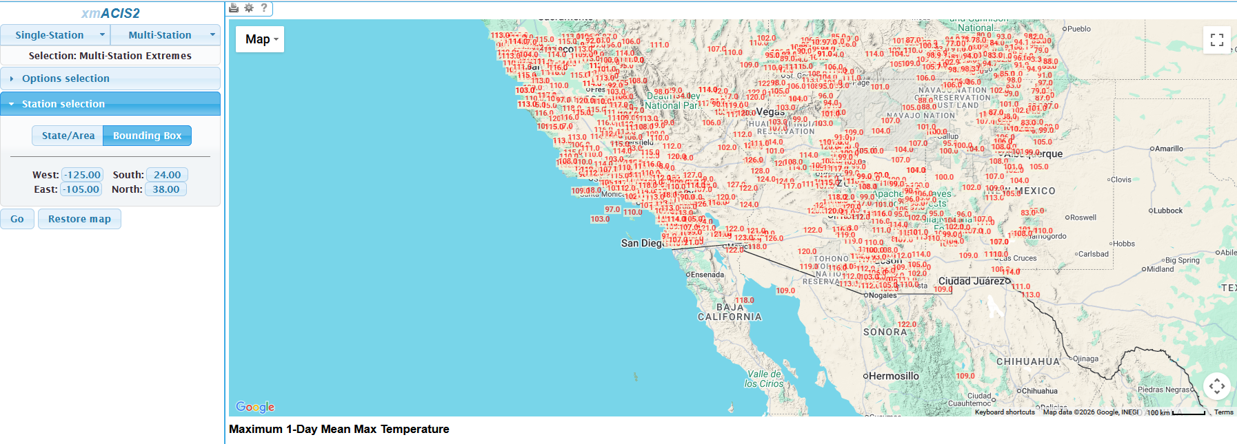
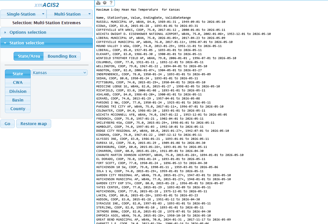
Notice that I select (under "Station Selection") a latitude-longitude bounding box. If this is too big, it won't let you create the map (and even at the size I selected, it took about a minute to create the map). You can also select individual states and some other geographical entities. There are other options to view the data, including the normal HTML and also CSV (the latter is useful if you do Python programming or other ways to manipulate the data). The example below shows the all-time January record high temperatures at all stations (only about half of them in this image since one must scroll down for the rest) in the XMACIS database in Kansas.
3. Iowa Environmental Mesonet (IEM):
Despite the name "Iowa", this website (https://mesonet.agron.iastate.edu/) allows one to view many products from not just Iowa but also the rest of the United States and, for that matter, the rest of the world. This is a huge website hosted by Iowa State, though again with a steep learning curve at the beginning. One can view an archive of many of the official observations (such as airport METARs) and also many of the National Weather Service products, including forecasts, going back to the 1990s (sometimes farther back). This is run by Daryl Herzmann, and he is quite creative with his programming skills (and fortunate enough to have a large server) to give us a myriad of ways to view the data. We will just look at a select few.
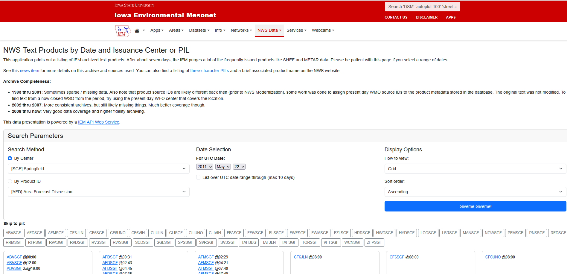
The first will be the NWS text products. This will include nearly all the text forecasts, watches, warnings, advisories, and Area Forecast Discussions, among many others. From the front page (not pictured here) just select the "NWS Data" pulldown and go to "Text Listing by WFO/Center/Product" or just go to https://mesonet.agron.iastate.edu/wx/afos/list.phtml. Yes, it includes NWS jargon, and you need to find the NWS office in the list (alphabetically by NWS office code) based on the location as this is oriented towards users who are well acquainted with the NWS structure.

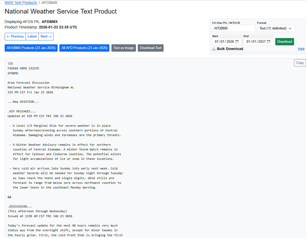
In the above image, I selected all the Area Forecast Discussions (AFD) for 23 Jan 2026 (note this is for UTC time, so 0000 UTC 23 Jan 2026 to 0000 UTC 24 Jan 2026 would be 6 PM CST 22 Jan 2026 to 6 PM CST 23 Jan 2026), shortly before the cold blast extended to the Gulf Coast and eventually through Florida and brought freezing rain and heavy snow to various parts of the Southeast. Here are the results.
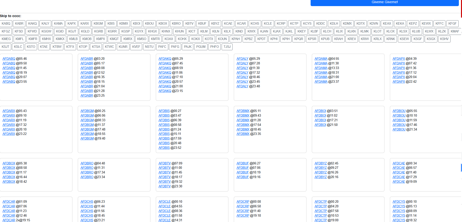
The above image was scrolled down to where you see a matrix with links to the products, named AFD plus the office code and time, so Birmingham, Alabama's code of AFDBMX would be the last six letters of the title, followed by the time issued in UTC (AFDBMX @ 2335) which would be 535 PM CST on 23 Jan 2026. I will select that one and get the product below.
With the same page as above, you can also select all products issued by an NWS office. We will look at the Springfield, Missouri (SGF) office on 22 May 2011, the day that Joplin, Missouri was devastated by an EF5 tornado which killed 158 people. After toggling and making the selection of the office under "By Center" and setting the correct date, you can see a list of products (though using the NWS coding)--with the screenshot showing only the first products.
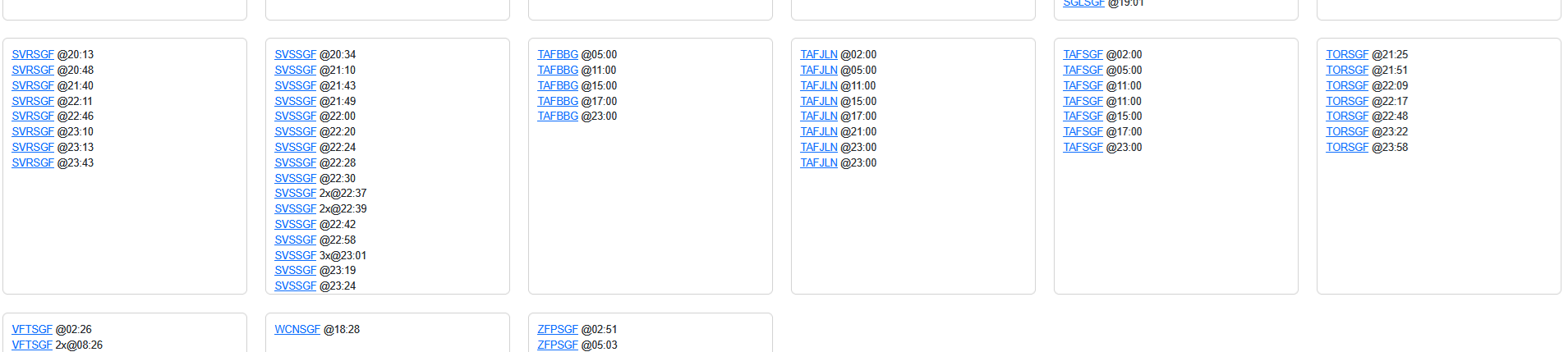
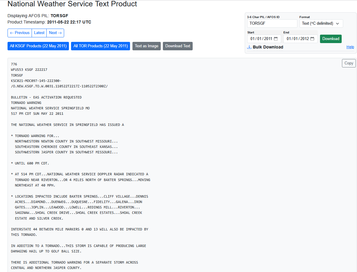
If you scroll down enough, you will find the tornado warnings which have the TOR code (plus SGF for the office code), so one would select TORSGF @ 2217 for the warning for the tornado that quickly developed just west of Joplin on the Kansas side of the Kansas-Missouri border and grew very large as it moved east into Joplin.
There are a lot of surface observations worldwide on the IEM website. It's not easy to find the page from the menu (but if you use the menu, go to the "Networks" pulldown, then select "ASOS/AWOS Airports" which will have the (predominantly airport) subcategory of observations called METARs. Then on the next page, go to "Historical Data" and then select "Download raw observations from the website". Or, it's easier just to go here: https://mesonet.agron.iastate.edu/request/download.phtml. You will get (scrolled down a bit) a page which looks like this:
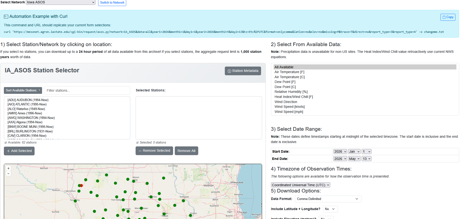
The important thing is to select the area of interest where it says "Select Network". Not only are US states and Canadian provinces listed but so are most foreign nations. Bolivia is one of those nations, and we will select "Bolivia ASOS" (in the scrolled down part below) and then select "[SLLP] La Paz (1936-now)" either in the selection box or on the map (zoomed in here). La Paz is actually El Alto International Airport, which is on a plateau above La Paz at an elevation of over 4000 meters (13000 feet), so it can get some strange weather. We will select "All Available" for the data (which will help those not used to seeing a RAW METAR observation). We will select "30 Nov 2012" to "1 Dec 2012" for the range of dates (note the data will end at 0000 UTC 1 Dec 2012, so if you wish to see data for 1 Dec 2012 as well, select the ending as 2 Dec 2012). One needs to scroll a bit beyond what this page shows to find the "Get Data" button down below (easy to find), which you would click.
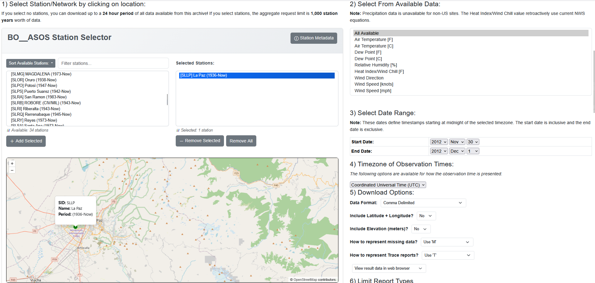
And we get this:
Since it's a CSV file, then you can see the data parsed out, based on the headers at the top. What's fascinating about this day is the thunderstorm in the middle of the day which brought a sudden drop in temperatures with snow (even though this was within a month of the Southern Hemisphere summer solstice), but then temperatures rose again shortly thereafter. The temperature at 1600 UTC (noon Bolivia Standard Time) was 46 F/8 C, but the temperature was down to 34 F/1 C just one hour later during the thunderstorm with snow. The temperature had returned to 45 F/7 C by 2200 UTC (6 PM Bolivia Standard Time), though that was still below the daytime high temperature of 53 F/12 C set at 1300 UTC or 9 AM. This output is a very compact way of looking at a lot of data, and with the CSV file, it's easy to incorporate that into a Python program too. Also, the IEM has fixed URLs, so you can easily manipulate a Python program to download a variety of data without using the user interface.
There is a lot of other data on IEM, but time and space on this page will stop us here, and we will move to the next site.
4. Space Science and Engineering Center (SSEC) Data Center:
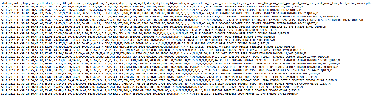
The SSEC Data Center at the University of Wisconsin is most notable for its extensive satellite images from the past. It can be found at https://www.ssec.wisc.edu/datacenter/archive.html with a menu driven archive. Most links from the front page take you to https://inventory.ssec.wisc.edu/inventory/, which looks like this:
There are two search options in the Search pulldown, one that says "Query" which we will use in a bit, and one that says "Calendar" which gives us some valuable information about the timing and region of the images but is only useful for downloading if you need large numbers of images. Below is a lot at what you get when you select "Calendar."

This is a matrix where you have time in the x-direction and the satellite in the y-direction. You can zoom out timewise by clicking on that "Time" button. Move the cursor over the dot, and you will see the part of the world that the images are centered on. Since the first satellites listed cover areas far from the US, you will need to scroll down to see other options.
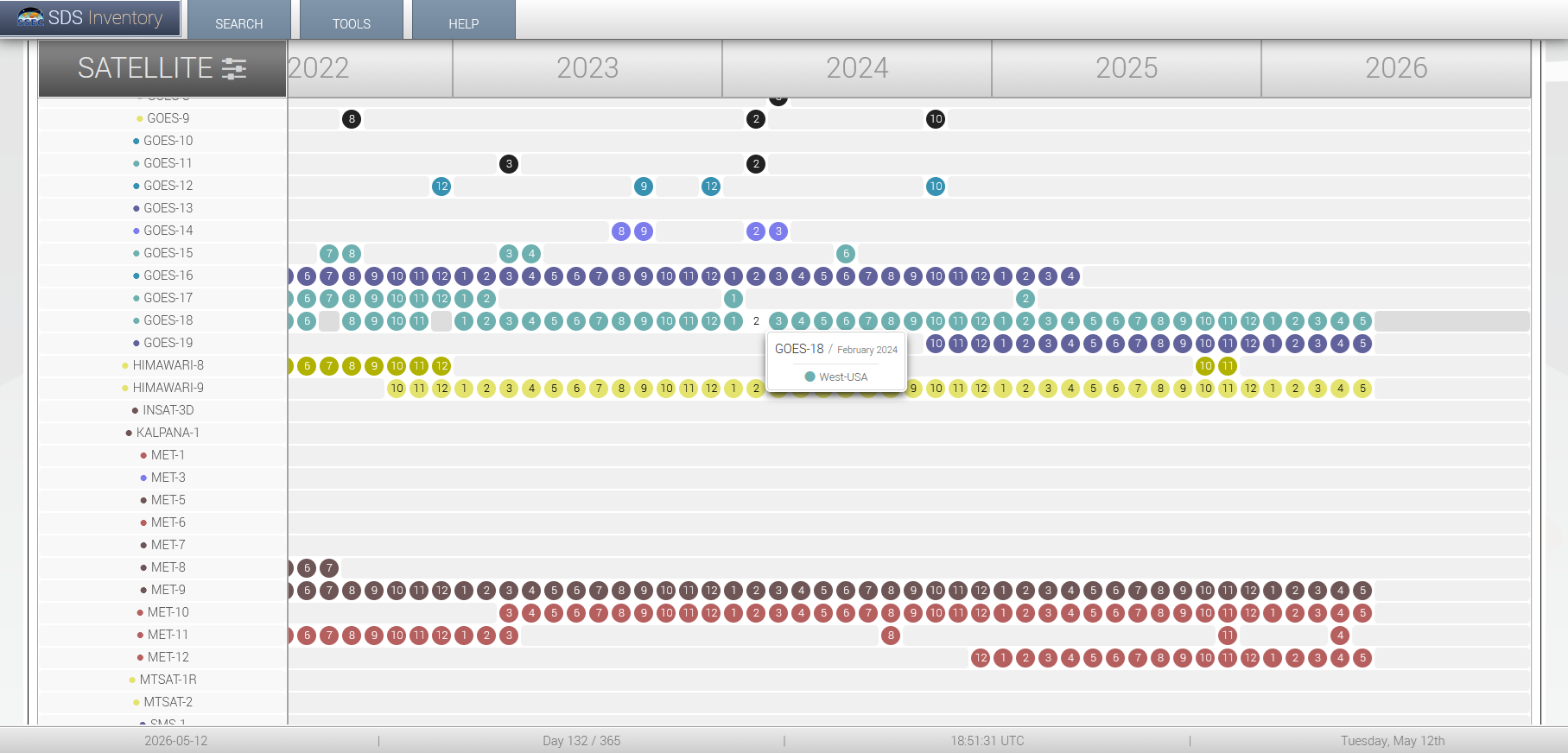
In this exercise, we will look at GOES-18 data, which covers the East Pacific and western North America (the label says "West USA" which is incomplete but still gives us an idea of what to look for). As a reminder, GOES-18 is geostationary, meaning it orbits the earth at a rate where it remains in the same location relative to the earth's geography as the earth rotates, and like all geostationary satellites, it is directly above the equator; in contrast, some satellites are polar orbiting, which have lower, faster orbits and vary their vantage points relative to earth's geography greatly during the orbit). Now that we have the basic timeline info from "Search"-->"Calendar" we will go to "Search"-->"Query" to look at satellite images.

The above is mostly intuitive, though remember that the time is in UTC, which is 8 (7) hours ahead of Pacific Standard (Daylight) Time and 5 (4) hours ahead of Eastern Standard (Daylight) Time. In many cases, you will have limited selections, though ABI (Advanced Baseline Imager) references the different spectral bands used for the images (more on that in a bit). While these images are low-resolution (a fraction of their original size due to storage limitations), you have some control over the area you see under "Coverage" (CONUS, which often displays just a part of the CONUS, vs. FD, or full-disk, and MESO1 and MESO2 which might focus on an area of significant weather). For this example, I am selecting 19 Aug 2023 for GOES-18 using the CONUS view. Next, you get the menu of images you can select.
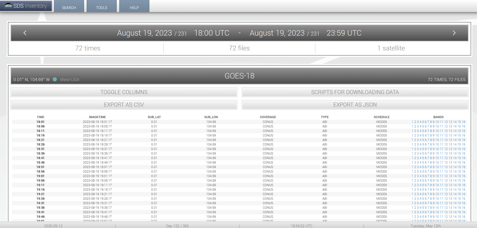
This is actually relatively basic if you focus on the time in the first column and the band in the last column. Generally, you would want to use Band 1 or 2 for visible imagery and Band 13 for infrared imagery. You can see the complete list of ABI bands and their specs here: https://www.goes-r.gov/mission/ABI-bands-quick-info.html.
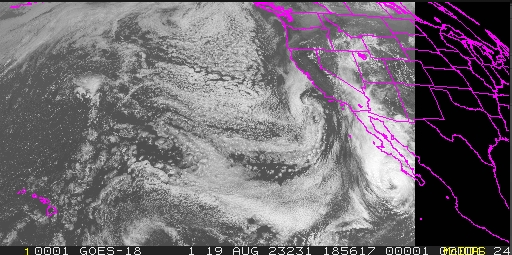
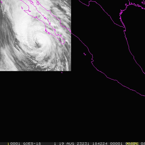
And now we have the part of the GOES-18 image from Hawaii to the western United States. And that happens to be Hurricane Hilary, on 19 Aug 2023, the day before the (barely non-tropical) remnants moved through southern California. The image appears small on the screen but can be magnified for better (but not full) resolution, like I have it here. Next, is another image from around the same time but for the full disk of the GOES-18.
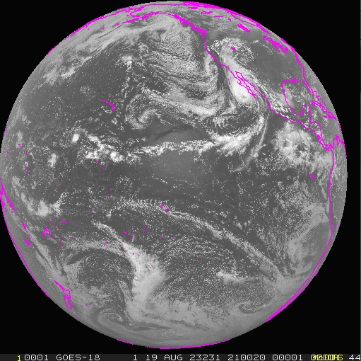
Finally, an image of Hurricane Hilary via the MESO1 option (definitely qualifies as a significant event to focus on!).
One thing to remember whenever using any data is that there is always a chance of bad data. One case: During the anomalous warmth in the south-central and central US this past December (2025), I was looking at all-time record high temperatures in Kansas, and found (in XMACIS) that Ashland, Kansas had a high temperature of 92 F/33 C on 30 Dec 1905. If that were true, that would be the all-time December highest temperature in Kansas. However, a look at (via XMACIS again) nearby high temperatures on 30 Dec 1905 showed mostly 40s with no stations in Kansas or neighboring Oklahoma above 57 F/14 C. Hmmm, sounds like that 92 F record should be thrown out. That is an example of an obvious record. The highest legitimate record in December is 90 F/32 C on 24 Dec 1955, also in Ashland and almost as high, but most other nearby stations in southwestern and south-central Kansas had highs well into the 80s (including 86 F/30 C at Dodge City), so this looks reasonable. Amazingly, Kansas (despite having generally cold winters, albeit quite variable) has reached 90 F/32 C in 11 of the 12 months of the year, with January being the only year to be absent of an official 90-degree reading (though about half the state has been 80 F/27 C or above before in January).
However, some meteorological data need more extensive research to consider, such as the 134 F/57 C reading from 10 Jul 1913 which is still officially the all-time world record. After doing research which included comparing nearby stations, a statistical analysis of the Death Valley temperature data, viewing the state of the atmosphere, and looking back at the equipment used, it appears that all the high-temperature readings taken in July 1913 at Death Valley were too high, probably by around 13 F/7 C. Here's the article: https://journals.ametsoc.org/view/journals/bams/107/1/BAMS-D-24-0313.1.xml. Note that, overall, I've seen more inaccurate data (such as from bad readings or incorrectly entered data) from outside the United States than within.
Hopefully, you can navigate these sites for weather statistics from the past. Perhaps in the future, I will do a blog entry for more "advanced" data (definitely I would discuss large datasets in binary format, especially those from NOAA or NASA websites). If you need any help, feel free to send me an email (note as a Certified Consulting Meteorologist, I'll be glad to answer any questions to point you in the right direction for free, but I would charge a fee if you need me to get you more extensive or difficult-to-retrieve data). And while most of the data are accurate, there are going to be the occasional observations that have an error (and likewise, if you have data which are in doubt which are important to you which are in doubt, I can investigate that as a consultant).
Come back soon for analyses of weather and climate, anywhere from California to other parts of the US to around the world!
Some of the future topics will include:
The wettest atmospheres in the world (based on "precipitable water")
Timberlines (highest elevation that trees can grow in a mountain range) and climate
Maximum precipitation rates reported given a certain temperature
Case studies of unusual storms